Near-Optimal and Tractable Estimation under Shift-Invariance

How hard is it to estimate a discrete-time signal $(x_{1}, ..., x_{n}) \in \mathbb{C}^n$ satisfying an unknown linear recurrence relation of order $s$ and observed in i.i.d. complex Gaussian noise? The class of all such signals is parametric but extremely rich: it contains all exponential polynomials over $\mathbb{C}$ with total degree $s$, including harmonic oscillations with $s$ arbitrary frequencies. Geometrically, this class corresponds to the projection onto $\mathbb{C}^{n}$ of the union of all shift-invariant subspaces of $\mathbb{C}^\mathbb{Z}$ of dimension $s$. We show that the statistical complexity of this class, as measured by the squared minimax radius of the $(1-\delta)$-confidence $\ell_2$-ball, is nearly the same as for the class of $s$-sparse signals, namely $O\left(s\log(en) + \log(\delta^{-1})\right) \cdot \log^2(es) \cdot \log(en/s).$ Moreover, the corresponding near-minimax estimator is tractable, and it can be used to build a test statistic with a near-minimax detection threshold in the associated detection problem. These statistical results rest upon an approximation-theoretic one: we show that finite-dimensional shift-invariant subspaces admit compactly supported reproducing kernels whose Fourier spectra have nearly the smallest possible $\ell_p$-norms, for all $p \in [1,+\infty]$ at once.

Nonconvex-Nonconcave Min-Max Optimization with a Small Maximization Domain

We study the problem of finding approximate first-order stationary points in optimization problems of the form $\min_{x \in X} \max_{y \in Y} f(x,y)$, where the sets $X,Y$ are convex and $Y$ is compact. The objective function $f$ is smooth, but assumed neither convex in $x$ nor concave in $y$. Our approach relies upon replacing the function $f(x,\cdot)$ with its $k$th order Taylor approximation (in $y$) and finding a near-stationary point in the resulting surrogate problem. To guarantee its success, we establish the following result: let the Euclidean diameter of $Y$ be small in terms of the target accuracy $\varepsilon$, namely $O(\varepsilon^{\frac{2}{k+1}})$ for $k \in \mathbb{N}$ and $O(\varepsilon)$ for $k = 0$, with the constant factors controlled by certain regularity parameters of $f$; then any $\varepsilon$-stationary point in the surrogate problem remains $O(\varepsilon)$-stationary for the initial problem. Moreover, we show that these upper bounds are nearly optimal: the aforementioned reduction provably fails when the diameter of $Y$ is larger. For $0 \le k \le 2$ the surrogate function can be efficiently maximized in $y$; our general approximation result then leads to efficient algorithms for finding a near-stationary point in nonconvex-nonconcave min-max problems, for which we also provide convergence guarantees.

Near-Optimal Model Discrimination with Non-Disclosure

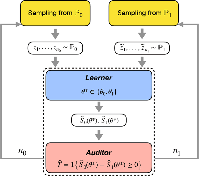
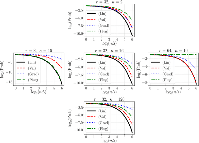
Let $\theta_0,\theta_1 \in \mathbb{R}^d$ be the population risk minimizers associated to some loss $\ell: \mathbb{R}^d \times \mathcal{Z} \to \mathbb{R}$ and two distributions $\mathbb{P}_0,\mathbb{P}_1$ on $\mathcal{Z}$. We pose the following question: Given i.i.d. samples from $\mathbb{P}_0$ and $\mathbb{P}_1$, what sample sizes are sufficient and necessary to distinguish between the two hypotheses $\theta^* = \theta_0$ and $\theta^* = \theta_1$ for given $\theta^* \in \{\theta_0, \theta_1\}$? Making the first steps towards answering this question in full generality, we first consider the case of a well-specified linear model with squared loss. Here we provide matching upper and lower bounds on the sample complexity, showing it to be $\min\{1/\Delta^2, \sqrt{r}/\Delta\}$ up to a constant factor, where $\Delta$ is a measure of separation between $\mathbb{P}_0$ and $\mathbb{P}_1$, and $r$ is the rank of the design covariance matrix. This bound is dimension-independent, and rank-independent for large enough separation. We then extend this result in two directions: (i) for the general parametric setup in asymptotic regime; (ii) for generalized linear models in the small-sample regime $n \le r$ and under weak moment assumptions. In both cases, we derive sample complexity bounds of a similar form, even under misspecification. Our testing procedures only access $\theta^*$ through a certain functional of empirical risk. In addition, the number of observations that allows to reach statistical confidence in our tests does not allow to "resolve" the two models -- that is, recover $\theta_0,\theta_1$ up to $O(\Delta)$ prediction accuracy. These two properties allow to apply our framework in applied tasks where one would like to \textit{identify} a prediction model, which can be proprietary, while guaranteeing that the model cannot be actually \textit{inferred} by the identifying agent.