Near-Optimal Model Discrimination with Non-Disclosure

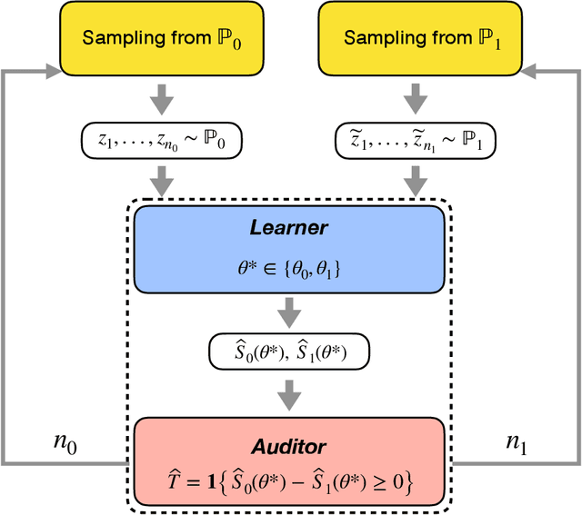
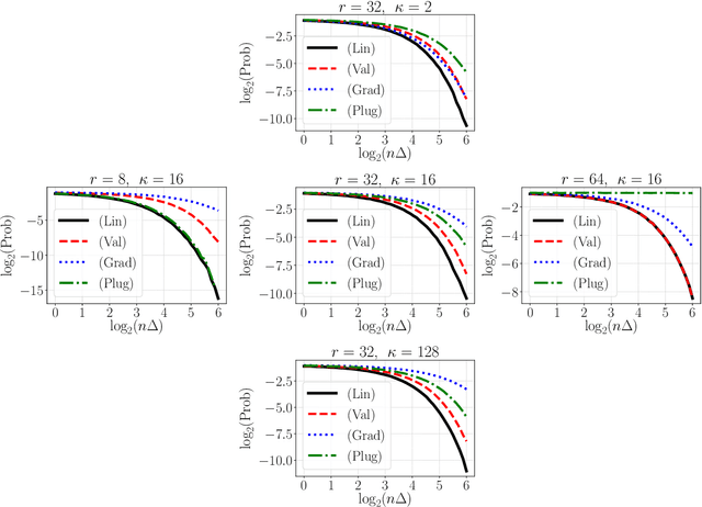
Let $\theta_0,\theta_1 \in \mathbb{R}^d$ be the population risk minimizers associated to some loss $\ell: \mathbb{R}^d \times \mathcal{Z} \to \mathbb{R}$ and two distributions $\mathbb{P}_0,\mathbb{P}_1$ on $\mathcal{Z}$. We pose the following question: Given i.i.d. samples from $\mathbb{P}_0$ and $\mathbb{P}_1$, what sample sizes are sufficient and necessary to distinguish between the two hypotheses $\theta^* = \theta_0$ and $\theta^* = \theta_1$ for given $\theta^* \in \{\theta_0, \theta_1\}$? Making the first steps towards answering this question in full generality, we first consider the case of a well-specified linear model with squared loss. Here we provide matching upper and lower bounds on the sample complexity, showing it to be $\min\{1/\Delta^2, \sqrt{r}/\Delta\}$ up to a constant factor, where $\Delta$ is a measure of separation between $\mathbb{P}_0$ and $\mathbb{P}_1$, and $r$ is the rank of the design covariance matrix. This bound is dimension-independent, and rank-independent for large enough separation. We then extend this result in two directions: (i) for the general parametric setup in asymptotic regime; (ii) for generalized linear models in the small-sample regime $n \le r$ and under weak moment assumptions. In both cases, we derive sample complexity bounds of a similar form, even under misspecification. Our testing procedures only access $\theta^*$ through a certain functional of empirical risk. In addition, the number of observations that allows to reach statistical confidence in our tests does not allow to "resolve" the two models -- that is, recover $\theta_0,\theta_1$ up to $O(\Delta)$ prediction accuracy. These two properties allow to apply our framework in applied tasks where one would like to \textit{identify} a prediction model, which can be proprietary, while guaranteeing that the model cannot be actually \textit{inferred} by the identifying agent.