Center-fixing of tropical cyclones using uncertainty-aware deep learning applied to high-temporal-resolution geostationary satellite imagery

Determining the location of a tropical cyclone's (TC) surface circulation center -- "center-fixing" -- is a critical first step in the TC-forecasting process, affecting current and future estimates of track, intensity, and structure. Despite a recent increase in the number of automated center-fixing methods, only one such method (ARCHER-2) is operational, and its best performance is achieved when using microwave or scatterometer data, which are not available at every forecast cycle. We develop a deep-learning algorithm called GeoCenter; it relies only on geostationary IR satellite imagery, which is available for all TC basins at high frequency (10-15 min) and low latency (< 10 min) during both day and night. GeoCenter ingests an animation (time series) of IR images, including 10 channels at lag times up to 3 hours. The animation is centered at a "first guess" location, offset from the true TC-center location by 48 km on average and sometimes > 100 km; GeoCenter is tasked with correcting this offset. On an independent testing dataset, GeoCenter achieves a mean/median/RMS (root mean square) error of 26.9/23.3/32.0 km for all systems, 25.7/22.3/30.5 km for tropical systems, and 15.7/13.6/18.6 km for category-2--5 hurricanes. These values are similar to ARCHER-2 errors when microwave or scatterometer data are available, and better than ARCHER-2 errors when only IR data are available. GeoCenter also performs skillful uncertainty quantification (UQ), producing a well calibrated ensemble of 200 TC-center locations. Furthermore, all predictors used by GeoCenter are available in real time, which would make GeoCenter easy to implement operationally every 10-15 min.

Distilling Machine Learning's Added Value: Pareto Fronts in Atmospheric Applications

While the added value of machine learning (ML) for weather and climate applications is measurable, explaining it remains challenging, especially for large deep learning models. Inspired by climate model hierarchies, we propose that a full hierarchy of Pareto-optimal models, defined within an appropriately determined error-complexity plane, can guide model development and help understand the models' added value. We demonstrate the use of Pareto fronts in atmospheric physics through three sample applications, with hierarchies ranging from semi-empirical models with minimal tunable parameters (simplest) to deep learning algorithms (most complex). First, in cloud cover parameterization, we find that neural networks identify nonlinear relationships between cloud cover and its thermodynamic environment, and assimilate previously neglected features such as vertical gradients in relative humidity that improve the representation of low cloud cover. This added value is condensed into a ten-parameter equation that rivals the performance of deep learning models. Second, we establish a ML model hierarchy for emulating shortwave radiative transfer, distilling the importance of bidirectional vertical connectivity for accurately representing absorption and scattering, especially for multiple cloud layers. Third, we emphasize the importance of convective organization information when modeling the relationship between tropical precipitation and its surrounding environment. We discuss the added value of temporal memory when high-resolution spatial information is unavailable, with implications for precipitation parameterization. Therefore, by comparing data-driven models directly with existing schemes using Pareto optimality, we promote process understanding by hierarchically unveiling system complexity, with the hope of improving the trustworthiness of ML models in atmospheric applications.

Can we integrate spatial verification methods into neural-network loss functions for atmospheric science?

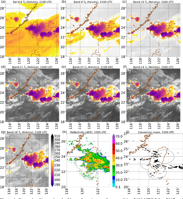
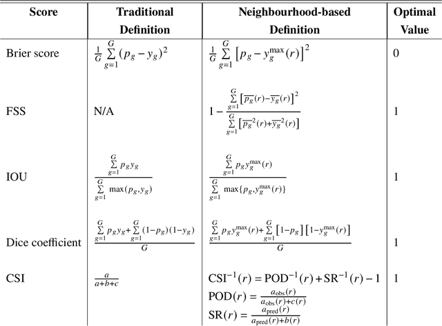
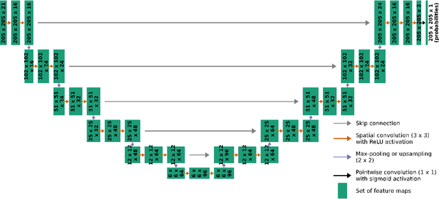
In the last decade, much work in atmospheric science has focused on spatial verification (SV) methods for gridded prediction, which overcome serious disadvantages of pixelwise verification. However, neural networks (NN) in atmospheric science are almost always trained to optimize pixelwise loss functions, even when ultimately assessed with SV methods. This establishes a disconnect between model verification during vs. after training. To address this issue, we develop spatially enhanced loss functions (SELF) and demonstrate their use for a real-world problem: predicting the occurrence of thunderstorms (henceforth, "convection") with NNs. In each SELF we use either a neighbourhood filter, which highlights convection at scales larger than a threshold, or a spectral filter (employing Fourier or wavelet decomposition), which is more flexible and highlights convection at scales between two thresholds. We use these filters to spatially enhance common verification scores, such as the Brier score. We train each NN with a different SELF and compare their performance at many scales of convection, from discrete storm cells to tropical cyclones. Among our many findings are that (a) for a low (high) risk threshold, the ideal SELF focuses on small (large) scales; (b) models trained with a pixelwise loss function perform surprisingly well; (c) however, models trained with a spectral filter produce better-calibrated probabilities than a pixelwise model. We provide a general guide to using SELFs, including technical challenges and the final Python code, as well as demonstrating their use for the convection problem. To our knowledge this is the most in-depth guide to SELFs in the geosciences.

CIRA Guide to Custom Loss Functions for Neural Networks in Environmental Sciences -- Version 1

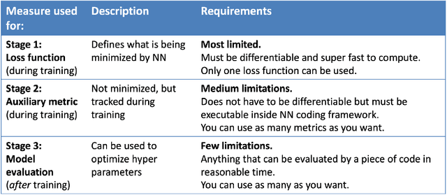
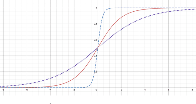
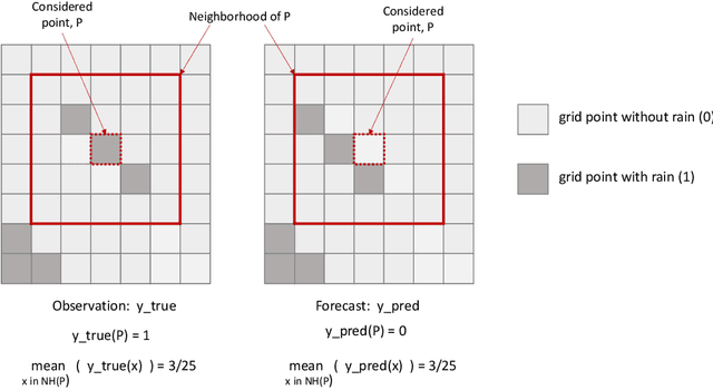
Neural networks are increasingly used in environmental science applications. Furthermore, neural network models are trained by minimizing a loss function, and it is crucial to choose the loss function very carefully for environmental science applications, as it determines what exactly is being optimized. Standard loss functions do not cover all the needs of the environmental sciences, which makes it important for scientists to be able to develop their own custom loss functions so that they can implement many of the classic performance measures already developed in environmental science, including measures developed for spatial model verification. However, there are very few resources available that cover the basics of custom loss function development comprehensively, and to the best of our knowledge none that focus on the needs of environmental scientists. This document seeks to fill this gap by providing a guide on how to write custom loss functions targeted toward environmental science applications. Topics include the basics of writing custom loss functions, common pitfalls, functions to use in loss functions, examples such as fractions skill score as loss function, how to incorporate physical constraints, discrete and soft discretization, and concepts such as focal, robust, and adaptive loss. While examples are currently provided in this guide for Python with Keras and the TensorFlow backend, the basic concepts also apply to other environments, such as Python with PyTorch. Similarly, while the sample loss functions provided here are from meteorology, these are just examples of how to create custom loss functions. Other fields in the environmental sciences have very similar needs for custom loss functions, e.g., for evaluating spatial forecasts effectively, and the concepts discussed here can be applied there as well. All code samples are provided in a GitHub repository.