Overview of Physics-Informed Machine Learning Inversion of Geophysical Data
Paper and Code
Oct 12, 2023


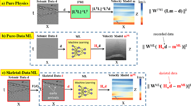
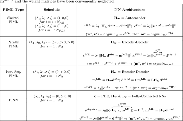
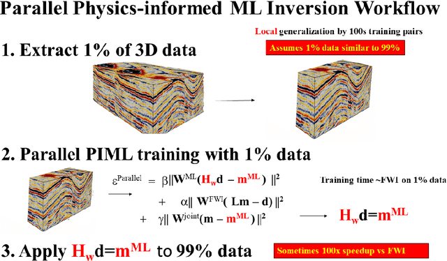
We review four types of algorithms for physics-informed machine learning (PIML) inversion of geophysical data. The unifying equation is given by the joint objective function $\epsilon$: \begin{eqnarray} \epsilon^{||-PIML}&=&\lambda_1 \overbrace{||{\bf W}^{ML}({\bf H}_{{\bf w}} {\bf d}^{obs}-{\bf m})||^2}^{NN} + \lambda_2 \overbrace{{||{\bf W}^{FWI}({\bf L} {\bf m}-{\bf d}^{obs})||^2}}^{FWI} ~+ \nonumber\\ \nonumber\\ && + ~~Regularizer, \label{PIML.eq120} \end{eqnarray}where the optimal model ${\bf m}^*$ and weights $\bf w^*$ minimize $\epsilon$. Here, The matrix weights are given by the boldface symbol $\bf W$, and full waveform inversion (FWI) is typically computed using a finite-difference solution of the wave equation, where $\bf L$ represents the forward modeling operation of the wave equation as a function of the model $\bf m$. Also, a fully-connected neural network (NN) is used to compute the model ${\bf H_w}{\bf d}^{obs} \approx \bf m$ from the observed input data ${\bf d}^{obs}$. The selection of weights $\lambda_i$ and the NN operations determine one of four different PIML algorithms. PIML offers potential advantages over standard FWI through its enhanced ability to avoid local minima and the option to locally train the inversion operator, minimizing the requirement for extensive training data for global applicability. However, the effectiveness of PIML relies on the similarity between the test and trained data. Nevertheless, a possible strategy to overcome this limitation involves initial pretraining of a PIML architecture with data from a broader region, followed by fine-tuning for specific data-a method reminiscent of the way large language models are pretrained and adapted for various tasks.
 Add to Chrome
 Add to Firefox
 Add to Edge